---

MS Excel: Two-Dimensional Lookup (Example #2)

This Excel tutorial explains how to perform a two-dimensional lookup (with screenshots and step-by-step instructions). This is example #2.

Question: I need to find the value on a chart (see below). The only problem is that I can have a material value that is not an exact match to a value on the chart. In this case, I need to round down and find the next smaller amount. For example, if I have 8 lbs of materials, it should return the value of 1 lbs of materials.

Answer: In effect, what we are trying to do is perform a 2-dimensional lookup in Excel. To find a value in Excel based on both a column and row value, you will need to use both a VLOOKUP function and a MATCH function.

Let's look at an example to see how you would use this function in a worksheet:

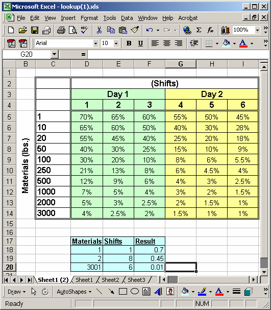
In the spreadsheet above, we have a listing of materials (in lbs.) and a listing of shift (1 through 6). What we want to do is find the correct value based on an amount of materials and a shift combination.

In the first case, we want to find the chart value for 1 lbs of materials and 1 shift. We've entered the following formula into cell F18:

=VLOOKUP(D18, $C$4:$I$14, IF(ISNA(MATCH(E18, $C$4:$I$4, 0)), 7, MATCH(E18, $C$4:$I$4, 0)), TRUE)

This formula returns 0.7 or 70%.

The last parameter on the VLOOKUP function is set to TRUE. This means that if the VLOOKUP does not find an exact match for the materials, it will look for the next smaller value. (In other words, rounding down)

Also, you'll find a 7 in the middle of the formula. This means that if you don't find a match for the shift value, it will use column (i) which is the 7th column. You'll have to modify this if you add more shifts.

In the second example, we are looking for the chart value for 2 lbs of materials and 8 shifts. We've entered the following formula into cell F19:

=VLOOKUP(D19, $C$4:$I$14, IF(ISNA(MATCH(E19, $C$4:$I$4, 0)), 7, MATCH(E19, $C$4:$I$4, 0)), TRUE)

This formula returns 0.45 or 45%.

In this example, an 8th shift can not be found, so the formula uses column (i) to derive the value.

In the final example, we are looking for the chart value for 3001 lbs of material and 6 shifts. We've entered the following formula in cell F20:

=VLOOKUP(D20,$C$4:$I$14,IF(ISNA(MATCH(E20,$C$4:$I$4,0)), 7,MATCH(E20,$C$4:$I$4,0)),TRUE)

This formula returns 0.01 or 1%.