MS Excel: How to use the SUMIF Function (WS)

This Excel tutorial explains how to use the Excel SUMIF function with syntax and examples.

Description

The SUMIF function is a worksheet function that adds all numbers in a range of cells based on one criteria (for example, is equal to 2000).

The SUMIF function is a built-in function in Excel that is categorized as a Math/Trig Function. It can be used as a worksheet function (WS) in Excel. As a worksheet function, the SUMIF function can be entered as part of a formula in a cell of a worksheet.

To add numbers in a range based on multiple criteria, try the SUMIFS function.

Subscribe

---

If you want to follow along with this tutorial, download the example spreadsheet.

Download Example

Syntax

The syntax for the SUMIF function in Microsoft Excel is:

SUMIF( range, criteria, [sum_range] )

Parameters or Arguments

range

The range of cells that you want to apply the criteria against.

criteria

The criteria used to determine which cells to add.

sum_range

Optional. It is the range of cells to sum together. If this parameter is omitted, it uses range as the sum_range.

Returns

The SUMIF function returns a numeric value.

Applies To

• Excel for Office 365, Excel 2019, Excel 2016, Excel 2013, Excel 2011 for Mac, Excel 2010, Excel 2007, Excel 2003, Excel XP, Excel 2000

Type of Function

• Worksheet function (WS)

Example (as Worksheet Function)

Let's explore how to use SUMIF as a worksheet function in Microsoft Excel.

Based on the Excel spreadsheet above, the following SUMIF examples would return:

=SUMIF(A2:A6, D2, C2:C6)
Result: 218.6   'Criteria is the value in cell D2

=SUMIF(A:A, D2, C:C)
Result: 218.6   'Criteria applies to all of column A (ie: A:A)

=SUMIF(A2:A6, 2003, C2:C6)
Result: 7.2     'Criteria is the number 2003

=SUMIF(A2:A6, ">=2001", C2:C6)
Result: 12.6    'Criteria is greater than or equal to 2001

=SUMIF(C2:C6, "<100")
Result: 31.2    'Adds values in C2:C6 that are less than 100 (3rd parameter is omitted)

Now, let's look at the example =SUMIF(A2:A6, D2, C2:C6) that returns a value of 218.6 and take a closer look why.

First Parameter

The first parameter in the SUMIF function is the range of cells that you want to apply the criteria against.

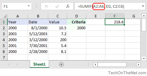
In this example, the first parameter is A2:A6. This is the range of cells that will be tested to determine if they meet the criteria.

Second Parameter

The second parameter in the SUMIF function is the criteria that will be applied against the range, A2:A6.

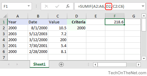
In this example, the second parameter is D2. This is a reference to the cell D2 which contains the numeric value, 2000. The SUMIF function will test each value in A2:A6 to see if it is equal to 2000.

Third Parameter

The third parameter in the SUMIF function is the range of numbers that will potentially be added together.

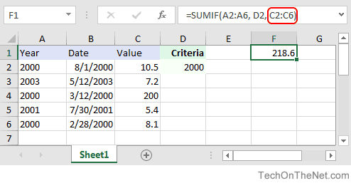
In this example, the third parameter is C2:C6. For every value in A2:A6 that matches D2, the corresponding value in C2:C6 will be summed.

Using Named Ranges

You can also use a named range in the SUMIF function. A named range is a descriptive name for a collection of cells or range in a worksheet. If you are unsure of how to setup a named range in your spreadsheet, read our tutorial on Adding a Named Range.

For example, if we created a named range called years in our spreadsheet that refers to cells A2:A6 in Sheet1 (Notice that the named range is an absolute reference that refers to =Sheet1!$A$2:$A$6 in the image below):

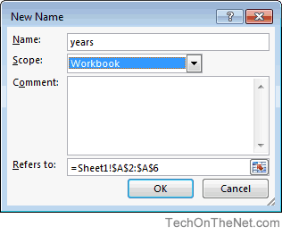
We could use this named range in our current example.

This would allow us to replace A2:A6 as the first parameter with the named range called years, as follows:

=SUMIF(A2:A6, D2, C2:C6)    'First parameter uses a standard range
Result: 218.6

=SUMIF(years, D2, C2:C6)    'First parameter uses a named range called years
Result: 218.6

Frequently Asked Questions

Question: I have a question about how to write the following formula in Excel.

I have a few cells, but I only need the sum of all the negative cells. So if I have 8 values, A1 to A8 and only A1, A4 and A6 are negative then I want B1 to be sum(A1,A4,A6).

Answer: You can use the SUMIF function to sum only the negative values as you described above. For example:

=SUMIF(A1:A8,"<0")

This formula would sum only the values in cells A1:A8 where the value is negative (ie: <0).

---

Question:In Microsoft Excel I'm trying to achieve the following with IF function:

If a value in any cell in column F is "food" then add the value of its corresponding cell in column G (eg a corresponding cell for F3 is G3). The IF function is performed in another cell altogether. I can do it for a single pair of cells but I don't know how to do it for an entire column. Could you help?

At the moment, I've got this:

=IF(F3="food"; G3; 0)

Answer:This formula can be created using the SUMIF formula instead of using the IF function:

=SUMIF(F1:F10,"=food",G1:G10)

This will evaluate the first 10 rows of data in your spreadsheet. You may need to adjust the ranges accordingly.

I notice that you separate your parameters with semi-colons, so you might need to replace the commas in the formula above with semi-colons.