

MS Excel 2003: Automatically alternate row colors (three shaded, three white)
This Excel tutorial explains how to use conditional formatting to automatically alternate row colors, three shaded and three white, in Excel 2003 and older versions (with screenshots and step-by-step instructions).
See solution in other versions of Excel:
Question: How can I set up alternating row colors in Microsoft Excel 2003/XP/2000/97? I want to alternate between 3 shaded rows and 3 white rows.
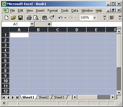
Answer: To do this, first highlight the rows that you wish to apply the formatting to. In this example, we've selected all rows in the spreadsheet.
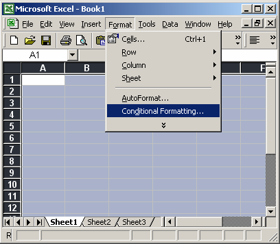
Under the Format menu, select Conditional Formatting.
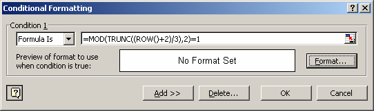
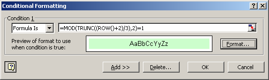
When the Conditional Formatting window appears, select "Formula Is" in the drop down. Then enter the following formula that uses the MOD, TRUNC and ROW functions:
=MOD(TRUNC((ROW()+2)/3),2)=1
You may need to adjust the ROW()+2 to either ROW() or ROW()+1 depending on which row you want to see shaded first.
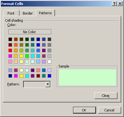
Next, we need to select the color we want to see in the shaded rows. To do this, click on the Format button.
When the Format Cells window appears, select the Patterns tab. Then select the color that you'd like to see. In this example, we've selected a light green. Then click on the OK button.
When you return to the Conditional Formatting window, you should see the following. Next, click on the OK button.
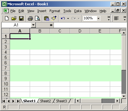
Now when you return to the spreadsheet, the conditional formatting will be applied.
As you can see, you now have alternating colors - 3 shaded rows followed by 3 white rows. You can insert, delete, and move rows, and you don't have to worry about reapplying formatting.
Advertisements