

MS Excel 2007: How to Show Bottom 10 Results in a Pivot Table
This Excel tutorial explains how to show the bottom 10 results in a pivot table in Excel 2007 (with screenshots and step-by-step instructions).
See solution in other versions of Excel:
Question: How do I show only the bottom 10 results in a pivot table in Microsoft Excel 2007?
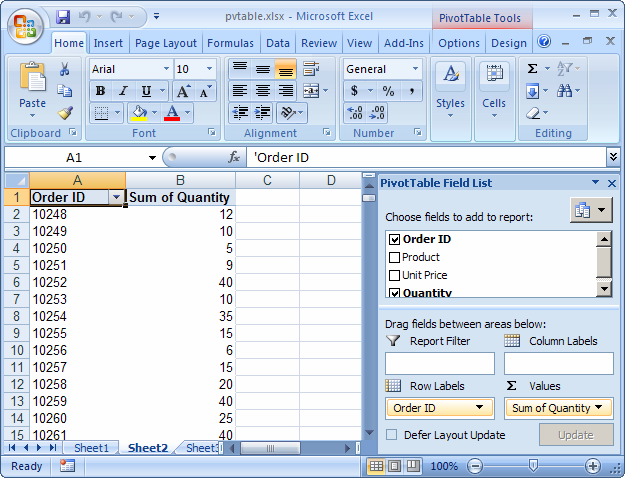
Answer: In this example, we want to see the bottom 10 Order IDs based on the "Sum of Quantity".
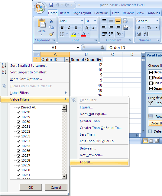
Click on the arrow to the right of the Order ID drop down box and select Value Filters > Top 10 from the popup menu.
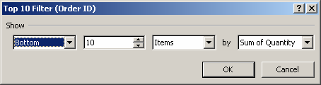
When the Top 10 Filter window appears, select Bottom, 10, Items, and Sum of Quantity in the respective drop downs. Then click on the OK button.
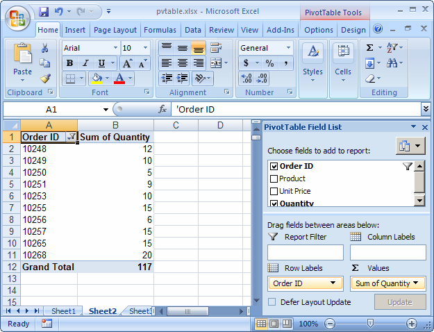
Now when you view your spreadsheet, you should only see the bottom 10 Order IDs based on the Sum of Quantity.


Advertisements