MS Excel: How to use the AGGREGATE Function (WS)

This Excel tutorial explains how to use the Excel AGGREGATE function with syntax and examples.

Description

The Microsoft Excel AGGREGATE function allows you to apply functions such AVERAGE, SUM, COUNT, MAX or MIN and ignore errors or hidden rows.

The AGGREGATE function is a built-in function in Excel that is categorized as a Math/Trig Function. It can be used as a worksheet function (WS) in Excel. As a worksheet function, the AGGREGATE function can be entered as part of a formula in a cell of a worksheet.

It was created by Microsoft to address the limitations of conditional formatting. Some conditional formatting can not be applied if there are errors in the range. The Excel AGGREGATE function allows you to ignore errors or hidden rows.

Syntax

There are 2 syntaxes for the AGGREGATE function:

REFERENCE Syntax

The REFERENCE syntax for the Microsoft Excel AGGREGATE function is:

AGGREGATE( function, options, reference1, [reference2], ... )

ARRAY Syntax

The ARRAY syntax for the Microsoft Excel AGGREGATE function is:

AGGREGATE( function, options, array, [optional_argument] )

Parameters or Arguments

function

The function that you wish to use and can be any of the following values:

Value	Explanation
1	AVERAGE
2	COUNT
3	COUNTA
4	MAX
5	MIN
6	PRODUCT
7	STDEV.S
8	STDEV.P
9	SUM
10	VAR.S
11	VAR.P
12	MEDIAN
13	MODE.SNGL
14	LARGE
15	SMALL
16	PERCENTILE.INC
17	QUARTILE.INC
18	PERCENTILE.EXC
19	QUARTILE.EXC

options

Specifies which values to ignore when applying the function to the range. If the options parameter is omitted, it assumes that options is set to 0. options can be any of the following values:

Value	Explanation
0	Ignore nested SUBTOTAL and AGGREGATE functions
1	Ignore nested SUBTOTAL, AGGREGATE functions, and hidden rows
2	Ignore nested SUBTOTAL, AGGREGATE functions, and error values
3	Ignore nested SUBTOTAL, AGGREGATE functions, hidden rows, and error values
4	Ignore nothing
5	Ignore hidden rows
6	Ignore error values
7	Ignore hidden rows and error values

reference1

The first numeric argument for the function when using the REFERENCE syntax.

reference2, ...

Optional. Numeric arguments 2 through 253 for the function when using the REFERENCE syntax.

array

An array, array formula, or reference to a range of cells when using the ARRAY syntax.

optional_argument

A second argument required if using the LARGE, SMALL, PERCENTILE.INC, QUARTILE.INC, PERCENTILE.EXC, or QUARTILE.EXC when using the ARRAY syntax.

Returns

The AGGREGATE function returns a numeric value.

Applies To

• Excel for Office 365, Excel 2019, Excel 2016, Excel 2013, Excel 2011 for Mac, Excel 2010

Type of Function

• Worksheet function (WS)

Example (as Worksheet Function)

Let's look at some Excel AGGREGATE function examples and explore how to use the AGGREGATE function as a worksheet function in Microsoft Excel:

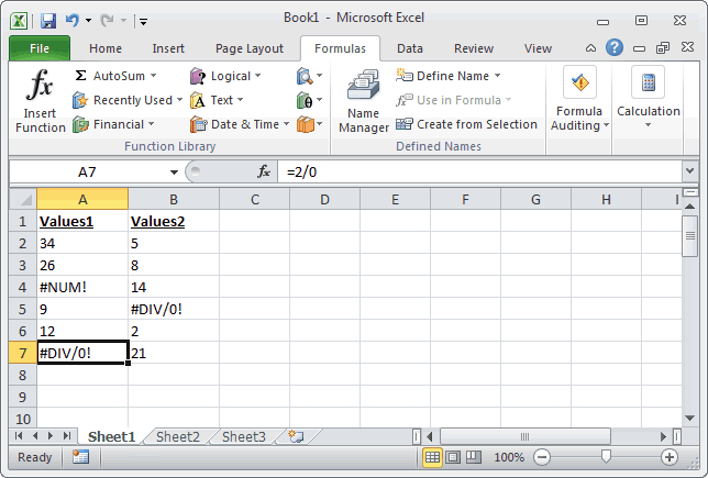
Let's look at a few examples based on the Excel spreadsheet above:

This first example (REFERENCE syntax) returns the AVERAGE for the range A2:A7 but ignores all error values. If you ran the AVERAGE(A2:A7) function directly, it would return #NUM! error because of the errors found in cells A4 and A7. The AGGREGATE function allows you to calculate an AVERAGE but ignore error values. The AGGREGATE function below would instead return 20.25 (instead of #NUM!).

=AGGREGATE(1, 6, A2:A7)

This next example (REFERENCE syntax) returns the MAX for the range A2:B7 but ignores all error values and hidden rows. If you ran the MAX(A2:B7) function directly, it would return #NUM! error because of the errors found in cells A4, A7, and B5. The AGGREGATE function allows you to calculate the MAX but ignore error values and hidden rows. The AGGREGATE function below would instead return 34 (instead of #NUM!).

=AGGREGATE(4, 7, A2:B7)

This final example (ARRAY syntax) uses LARGE to return the 2nd largest value for the range A2:B7 but ignores all error values. If you ran the LARGE(A2:B7,2) function directly, it would return #NUM! error because of the errors found in cells A4, A7, and B5. The AGGREGATE function allows you to calculate the 2nd LARGEST value but ignore error values. The AGGREGATE function below would instead return 26 (instead of #NUM!).

=AGGREGATE(14, 6, A2:B7, 2)